
Satellite Image Bands
So-called passive satellite systems record the part of the solar radiation that is reflected from the observed objects, in most cases features on the Earth surface. Satellites acquire data in specific spectral bands, parts of the electromagnetic spectrum that can be characterised by a central wavelength and a bandwidth.
Optical satellites are operating in the range from the visible part of the spectrum (wavelength 400-700 nm) to the infrared part (from the so-called Near Infrared, NIR, from 700 nm to 2 µm, and Middle Infrared, MIR, from 2 to 5 µm, to Far Infrared, FIR, 25 to 1000 µm). A special part of the infrared spectrum is the Thermal Infrared, TIR, with wavelengths between 3 and 25 µm.
The human eye has receptors that are sensitive for radiation in the blue, green, and red parts of the spectrum. We see objects in different colours depending on differences in the light emission or reflection by these objects. In the same way objects on the Earth’s surface reflect sunlight differently depending on the material they consist of and on its status.
The examples show image bands of the satellite Sentinel-2, which acquires data in bands with central wavelengths ranging from 443 nm to 2.19 µm. For comparison, a true-colour image prepared from the bands in the visible range of the spectrum has been added on the next page to make the interpretation of the visible objects easier.
Comparison with the true-colour image shows, why the sea water appears in blue – especially the blue band is relatively bright, while in the red band the water appears dark. Combined, this results in a light blue colour. Similar considerations can be made with other landcover classes: forests, fields, cropland, and built-up areas such as towns and traffic infrastructure (look at the airport Fiumicino to the left of the images!).
The human eye and mind are very efficient with respect to interpreting true-colour images. Special algorithms applied to the data allow to extract a wealth of additional information that would not be accessible to the human perception otherwise.
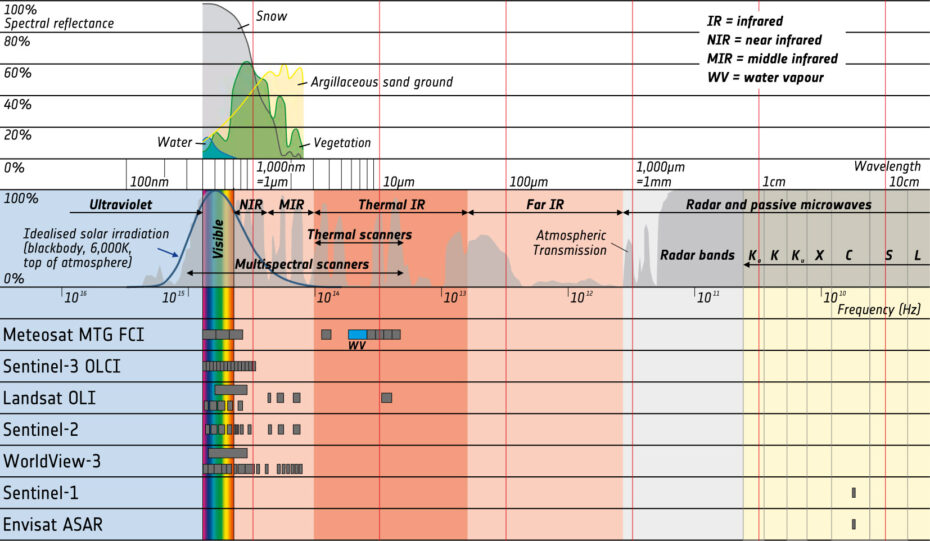
Diagram showing the electromagnetic spectrum, reflectance curves for selected land cover classes (top), the atmospheric transmission (middle), and where the bands of selected satellites are located (bottom). Note: the x-axis is logarithmic, i.e. with each red line the wavelength increases by a factor of 10.
Exercises
- Satellite Map:
- Use the layer selector to look at the different satellite bands of the Sentinel-2 data. Compare them with the true-colour image and try to identify the land use and landcover classes in the region.
- Try to identify forests (note: forests appear in dark green or brown colours, e.g. in the lower centre of the images; therefore, they are dark in the visible bands).
- Look at the water bodies (sea, river). How do they appear in the individual image bands?
- For advanced readers: compare the land cover classes identified in the images (especially water and vegetation) with the spectral reflectance curves in the upper part of the diagram below and describe your findings (the grey boxes in the line “Sentinel-2” indicate the locations of the bands, band index starting with 1 for the leftmost band).
- Copernicus Browser:
- Open the case study area in the Copernicus Browser.
- Find the most recent Sentinel-2 dataset covering the area displayed in the satellite map.
- Select a natural colour representation.
- Can you identify additional, recent changes in the area?
- Select the false colour infrared representation. Can you identify the land-use of the most intensely vegetated areas (represented by bright red colours)?
- Select the custom visualisation. Visualize individual bands (you can do this by dragging the same band to R, G, and B fields). Do this for different bands and compare. What are your findings with respect to the representation of different landcover classes (water, agricultural land, built-up land, etc.)?
Links and Sources
| Downloads: | |
|
PDF document of the case study (includes exercises): English, German, French, Italian, Spanish |
|
|
|
This case study is covered on page 18 of the printed ESA Schoolatlas – download the PDF document of the page: English, German, French, Italian, Spanish |
| Links: |
|